这是一篇来自美国的关于分子动力学项目的代码代写
The aim of the project is to develop code to run an elementary molecular dynamics (MD) simulation. MD simulations are widely used in computational chemistry, physics, biology, material science etc. It was also one of the first scientific uses of computers going back to work by Alder and Wainwright who, in 1957, simulated the motion of about 150 argon atoms. (See Alder, B. J. and Wainwright, T. E. J. Chem. Phys.
27, 1208 (1957) and J. Chem. Phys. 31, 459 (1959))
In MD, each atom is represented as a point in space. The atoms interact with each other via pairwise potentials, in a similar manner to the way gravity interacts between the planets, sun, moons and stars. In practice this is just an approximation since quantum effects are often important – but we’ll ignore this and confine our discussions to “classical” MD.
To calculate the potential energy between two atoms and , we will use a Lennard-Jones potential energy function of the form where rij is the distance between the two atoms. [Note: For simplicity we here choose the Lennard-Jones interaction parameters A=1 and ]. To evaluate the interaction for many bodies we must simply perform a sum over all unique two body interactions. For example,for 3 particles we will have interactions 1-2, 1-3 and 2-3.
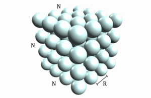
In this program we will start with a grid of stationary atoms arranged in a cubic box with N atoms along each side, such that there are a total of atoms as shown in the following figure, with adjacent atoms separated by a distance R .
Getting Started
To get started working on this assignment, fork this repository and then clone your copy of the repository (with URL https://gitlab.cecs.anu.edu.au/<YOUR_UID>/comp3320-2022-assignment-1 ) to a folder on Gadi, just as you did with the labs.
Navigating the Repo
You will notice that the repository already contains a number of files with template code that has been written for you. It is not a requirement that you keep or use any of this code, but it is there to help structure your program and the general usage of the program must remain the same. Here is a brief overview of the files in this repo:
- img/ – this folder contains the images used in this document.
- lib/ – this folder contains some useful library code and classes for the python program. You should be able to complete the assignment without modifying these files, however you may want to look at them to understand how they work and to be able to modify them if you wish.
- argument_parser.py – Reads in the arguments for md.py.
- c_structures.py – Defines C data structures for the python/C interface.
- utils.py – Defines a 3D vector class and an Atom class.
- visual_atom.py – Defines an Atom subclass which provides visualization.
- .gitignore – this file tells git which files it can safely ignore, such as your compiled executables.
- Makefile – this file is used to compile the C code.
- README.md – these instructions!
- Report.pdf – you should replace this pdf with your report to complete Step 3 below.
- WRITEUP.txt – you should fill out this file with details of how long you spent on each component of the assignment, any notable deficiencies in your work and detail any collaboration.
- md.py – this is the main python program which you must complete in Step 1 and provides a visualization of your simulation for use in debugging if you wish.
- md_AoS.c – this is a C version of md.py for use with the AoS code written in Step 2 without visualization. This may be useful for making performance measurements of your code.
- md_SoA.c – this is a C version of md.py for use with the SoA code written in Step 2 without visualization. This may be useful for making performance measurements of your code.
- md_lib_AoS.c – this contains the C code with an AoS data structure that you will write in Step 2 that is called by both md.py and md_AoS.c .
- md_lib_SoA.c – this contains the C code with an SoA data structure that you will write in Step 2 that is called by both md.py and md_SoA.c .
- sample_outputs.md – this provide some sample outputs that your code should produce to check you are on the right track.
- auto_test.py – this is a test script to help you make sure that your code will pass the auto marker
The main program has 4 positional arguments
- – number of atoms in each dimension of the box,
- – the spacing between adjacent atoms in the grid,
- – the time step, and
- – the number of time steps in your simulation.
There are also two optional arguments provided with the -v and -c flags respectively. The -v flag enables the visualization (this will not work on Gadi) and the -c flag followed by an additional parameter instructs the program to use one of your C implementations for the compute intensive portions of the program rather than the python code. For example -c AoS instructs the program to outsource the compute-intensive functions to the code in md_lib_AoS.c (provided it has been compiled to md_lib_AoS.so via the make command).
The python program input is as follows: python3 md.py N R dt iter [-v] [-c {AoS, SoA, Opt}] . You can obtain this information by
running python3 md.py –help .
You are also provided with two C programs ( md_AoS and md_SoA ) to help measure the performance of your C code which you will write in Step 2 ). These can be run with ./md_AoS N R dt iter and ./md_SoA N R dt iter respectively. You can compile all of the C code by running the command make .
Running the code on Gadi
To run the python code on Gadi, you will first need to load the python3/3.8.5 module by running the command
module load python3/3.8.5
You can then check that everything is working by running the command python3 md.py 1 1 0.001 1 which should give the output
Initial grid spacing : 1.000000
Total number of atoms : 1
Integration time step : 0.001000
Number of timesteps : 1
TIME Total Kinetic Potential
—————————————————–
0.000000 0.000000e+00 0.000000e+00 0.000000e+00
The C code can be run as usual without loading additional modules.
Running the code with visualization
You can also clone your copy of the repository to your own machine which will allow you to view a 3D visualization of the simulation in your browser. This is NOT a requirement to complete the assignment and we will not test the visualization when marking, it is only provided to assist in debugging your program (and it is cool to watch your simulation in real time!).